Interrogate parameter space
Reveal how boundary conditions, coupled variables, and uncertainty reshape the feasible region.
Computational visualization
Skar translates mathematics, physics-informed models, and simulation data into visual structures that expose geometry, dynamics, uncertainty, stability, and constraint.
From governing structure to physical intuition
A simulation can produce an answer while concealing the mechanism that produced it. We construct visual representations of state space, phase evolution, boundary conditions, coupled modes, and stochastic convergence so technical behavior can be inspected rather than merely reported.
Visualization becomes part of the analytical method: a way to interrogate sensitivity, compare parameter regimes, expose instability, and communicate why a conclusion remains physically and mathematically defensible.
Reveal how boundary conditions, coupled variables, and uncertainty reshape the feasible region.
Distinguish transient behavior from stable modes, periodic structure, and the variables controlling system response.
Preserve the chain from governing assumptions and equations through observed behavior and a defensible decision.
Analytical environments
High-dimensional systems are governed by interacting constraints, nonlinear response, uncertainty, and path dependence. We build computational views that preserve those relationships while making the governing behavior possible to examine.
Vary initial conditions, boundary conditions, and coupled parameters to locate sensitivity, stability, and feasible operating regions.
Track state evolution, modal behavior, constraint interaction, and the propagation of disturbances through a system.
Connect model assumptions, numerical experiments, uncertainty, and observed behavior in one inspectable analytical record.
Uncertainty quantification begins with an ensemble, not a single deterministic path. Each particle represents a sampled state drawn from a broader distribution of possible conditions.
As the ensemble evolves, individual trajectories remain distinct while their occupancy converges toward a coherent manifold. The distribution—not one privileged sample—becomes the object of analysis.
The resulting structure exposes range, concentration, outliers, and the assumptions capable of moving the system into a different regime.
Computational study · Procedural terrain
Layered trigonometric detail forms a continuous mountain landscape. Movement through the field reveals ridges, depth, and changing perspective.
Procedural terrain requires WebGL to display.
Computational studies
These are live equations evaluated in the browser at every frame—not prerecorded animations. Together they render cyclic symmetry, driven ensembles, constrained surfaces, coupled phase modes, stochastic transport, and topology through continuous state space.
Seven parameterized branches form a cyclically symmetric field. A traveling phase perturbation modulates curvature and radius while the global mode remains coherent—an analogue for synchronized oscillators, rotating machinery, and periodic loading.
Twenty thousand sample points evolve under a shared nonlinear phase law. Local trajectories remain distinct while macroscopic structure emerges, illustrating coherent response in many-body systems, network dynamics, and distributed control.
Stacked parametric sections reconstruct a deforming surface of revolution. Changes in waist, curvature, and modal amplitude show how boundary conditions restrict the admissible geometry of a design or physical system.
Two phase-shifted parametric bodies move within one nonlinear field. Their shared governing law preserves coherence while relative position changes—an analogue for coupled oscillators, interacting states, and second-order dependency.
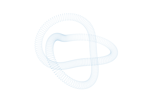
Nested trigonometric forcing produces two related structures that exchange phase and orientation. Continuous deformation reveals mode coupling and adaptive response without breaking the topology of the system.
Two ribbon manifolds evolve along a 1:2 Lissajous trajectory. Normal-direction perturbations generate local deformation while the orbit remains closed, clarifying periodic transport, handoffs, and stability through a complete state cycle.
Lagrangian tracers evolve through a time-varying, divergence-free velocity field while stochastic diffusion separates neighboring paths. The resulting density reveals coherent transport barriers, mixing regions, and the rate at which initial certainty is lost.
A dense ribbon is transported around a (3,8) torus knot. Slow orbital motion exposes periodic closure, winding number, and the continuous local frame that turns a one-dimensional trajectory into an oriented surface without changing its topology.
Interactive visualization
Move your pointer across the canvas to guide the flowing strands.
This interactive field requires motion effects and WebGL to be available.